Over my two decades of experience in robotics and engineering, I’ve found LiDARs to be integral part of how I’ve used robotic systems. I’ve used LiDARs for applications ranging from localization and mapping to obstacle avoidance, safety systems, and ground truth tracking. Most of the LiDARs I’ve used have been industrial grade devices, and today I have a hobbyist grade LiDAR that I need to get running before I put it on a home project. This presents me with an opportunity to finally explore Holoviews and Panel using some high-frequency real-time sensor data.
In exploring new technologies and tools within the data visualization and dashboard creation space, my curiosity is continually drawn to Holoviews and Panel. Holoviews is a Python library designed to simplify data visualization and is capable of using different backends, including Matplotlib and Bokeh. Panel is, like Holoviews, part of the Holoviz system and is a high-level dashboarding solution, allowing users to create interactive, web-based applications.
What sets Holoviews and Panel apart from commercial options like Plotly and Streamlit is their robust, community-driven open-source ethos. For personal projects, I will always give preference to community driven Free/Libre Open Source Software.
The technical underpinnings of Panel also offer a compelling case for its adoption over alternatives. My experience with Streamlit, while incredibly positive, has been tempered by its stateless model. Streamlit’s approach, where the app’s state is not preserved between user interactions, causing the entire script to rerun with every action, can be less than ideal. This model often results in performance bottlenecks, particularly in data-intensive applications common in my work. Panel, on the other hand, utilizes a stateful model, allowing for partial updates and, crucially, more efficient handling of live data streams.
Testing this LiDAR gave me a perfect excuse to explore the capabilities of Holoviews and Panel. I am particularly interested in how the plotting interfaces feel, how much boilerplate Panel needs to get something running, and how performant the visualizations and dashboards can be with a real-time data stream.
Setting Up the LiDAR System
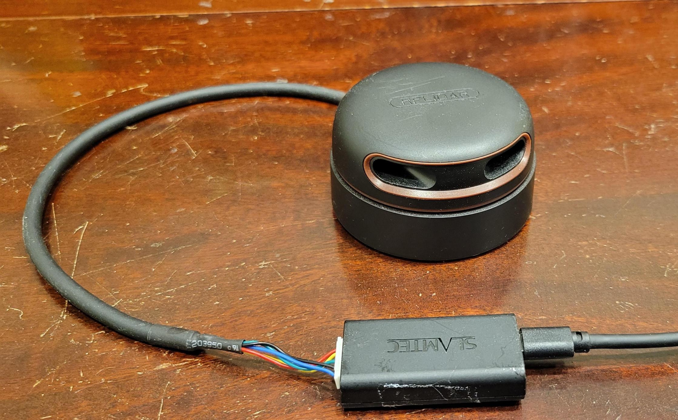
The LiDAR is a Slamtec RPLiDAR A2M8. It is a 2D 360° scanner with an 8-meter range. It can scan at 5-15 Hz and has an angular resolution of 0.9° at 10 Hz. When working with any sensor, the first thing you should do is pull up the data sheets and manuals! In this case, it is a straight-forward and easy to use sensor that has a number of options for using it. There’s a ROS (Robotic Operating System) driver, which appears to be the most popular way to interface, but that’s not appropriate for my project. I don’t need to use a library, but PyRPlidar appears to be a solid implementation of the protocol and will save us time getting started.
The first step is to plug the scanner into the computer and see if it shows up. Using a Linux computer, which all instructions will assume, the most basic way to check is to run $ sudo dmesg to get some information about the device and see where it has attached.
$ sudo dmesg
[...]
[86398.0045891] usb 5-4: New USB device found, idVendor=10c4, idProduct=ea60, bcdDevice= 1.00
[86398.045898] usb 5-4: New USB device strings: Mfr=1, Product=2, SerialNumber=3
[86398.045901] usb 5-4: Product: CP2102 USB to UART Bridge Controller
[86398.045905] usb 5-4: Manufacturer: Silicon Labs
[86398.045908] usb 5-4: SerialNumber: 0001
[86398.075170] usbcore: registered new interface driver usbserial_generic
[86398.075183] usbserial: USB Serial support registered for generic
[86398.076474] usbcore: registered new interface driver cp210x
[86398.076486] usbserial: USB Serial support registered for cp210x
[86398.076525] cp210x 5-4:1.0: cp210x converter detected
[86398.080941] usb 5-4: cp210x converter now attached to ttyUSB0
Since I am accessing the device on a tty* I need to be in the dialout group. I run $ groups and see that my user is not in this group. I add it with:
$ sudo usermod -aG dialout $USER
It is important to note that this change does not take effect immediately. Shells, and even your GUI login, need to be restarted for changes to your user’s groups to take effect. You can forge ahead in your open shell on most systems by calling $ newgrp. This step often trips up many people, especially those not fluent in Linux. This is not hard stuff but can be quite tricky if you’ve never seen it before.
Next, because I don’t like accessing the device over a name that can change, I will map this specific LiDAR to a static name. Using the dmesg output information above, I run
$ echo 'SUBSYSTEM=="tty", ATTRS{idVendor}=="10c4", ATTRS{idProduct}=="ea60", MODE:="0660", GROUP:="dialout", SYMLINK+="rpLiDAR"' | sudo tee /etc/udev/rules.d/99-rpLiDAR.rules
$ sudo udevadm control --reload-rules
$ sudo udevadm trigger
Now, anytime I plug the LiDAR in, I can access it on /dev/rpLiDAR, even if something else happened to attach to ttyUSB0 first.
Since I’ve already decided I’ll use Python and the PyRPlidar package, it is prudent for us to set up a Python virtual environment and install support libraries. There are too many “good enough” ways to manage Python virtual environments to go into details here. Suffice it to say, use Python virtual environments. Solely because this is the computer I am on, I will proceed with Anaconda and the conda command. I used the following commands, with output removed:
$ conda create -n rpLiDAR python=3.11
$ conda install pytest pyserial panel hvplot
And the library I chose to use is not in Anaconda, so I will use pip to install it
$ pip install PyRPlidar
First LiDAR Comms
I’m a believer in Gall’s Law:
A complex system that works is invariably found to have evolved from a simple system that worked.
With Galls’ Law in mind, I chose to connect to the LiDAR as quickly as possible and get information back. Hackers will start with Minicom. Most people in the modern era working with these tools will likely fire up Jupyter Lab and iterate from simple working to more complex working. For this work, I chose to use Emacs org-mode.
The first question to answer is can I communicate with the device at all?
So, moving over to Python and focusing on communication through my chosen library, I run the following code:
from PyRPlidar import PyRPlidar

# this config info be used a lot so break it out early
rp_cfg = {
    'port': '/dev/rpLiDAR',
    'baudrate': 115200,
    'timeout': 3,
}
LiDAR = PyRPlidar()
LiDAR.connect(**rp_cfg)
info = LiDAR.get_info()
print(f"LiDAR information:\n{info}\n")
health = LiDAR.get_health()
print(f"LiDAR health:\n{health}\n")
samplerate = LiDAR.get_samplerate()
print(f"LiDAR sample rate: {samplerate}\n")
scan_modes = LiDAR.get_scan_modes()
print("Scan modes:\n")
for scan_mode in scan_modes:
    print(scan_mode)
LiDAR.disconnect()
Executing this yields the following (successful!) output:
PyRPlidar Info : device is connected
LiDAR information:
{'model': 40, 'firmware_minor': 25, 'firmware_major': 1, 'hardware': 5, 'serialnumber': 'B4889AF2C1EA9FC0BEEB9CF33B5B3200'}
LiDAR health:
{'status': 0, 'error_code': 0}
LiDAR sample rate: {'t_standard': 500, 't_express': 250}
{'name': 'Standard', 'max_distance': 3072, 'us_per_sample': 128000, 'ans_type': 'NORMAL'}
{'name': 'Express', 'max_distance': 3072, 'us_per_sample': 64000, 'ans_type': 'CAPSULED'}
{'name': 'Boost', 'max_distance': 3072, 'us_per_sample': 32000, 'ans_type': 'ULTRA_CAPSULED'}
Scan modes:
{'name': 'Standard', 'max_distance': 3072, 'us_per_sample': 128000, 'ans_type': 'NORMAL'}
{'name': 'Express', 'max_distance': 3072, 'us_per_sample': 64000, 'ans_type': 'CAPSULED'}
{'name': 'Boost', 'max_distance': 3072, 'us_per_sample': 32000, 'ans_type': 'ULTRA_CAPSULED'}
PyRPlidar Info : device is disconnected
After confirming the library, which has not been maintained in quite a while, still works with my LiDAR, it was time to capture some scans.
import time

def simple_scan(rp_cfg):
    LiDAR = PyRPlidar()
    LiDAR.connect(**rp_cfg)
    try:
        samplerate = LiDAR.get_samplerate()
        LiDAR.set_motor_pwm(samplerate.t_standard)
        time.sleep(2)
        scan_generator = LiDAR.force_scan()
        for count, scan in enumerate(scan_generator()):
            print(count, scan)
            if count == 360: break
    finally:
        LiDAR.stop()
        LiDAR.set_motor_pwm(0)
        LiDAR.disconnect()
simple_scan(rp_cfg)
Running this in my org-mode source code block returns:
PyRPlidar Info : device is connected
0 {'start_flag': False, 'quality': 0, 'angle': 312.65625, 'distance': 0.0}
1 {'start_flag': False, 'quality': 15, 'angle': 337.1875, 'distance': 0.0}
2 {'start_flag': False, 'quality': 15, 'angle': 332.234375, 'distance': 929.0}
3 {'start_flag': False, 'quality': 15, 'angle': 333.765625, 'distance': 921.0}
4 {'start_flag': False, 'quality': 15, 'angle': 335.203125, 'distance': 912.5}
5 {'start_flag': False, 'quality': 15, 'angle': 336.640625, 'distance': 905.75}
6 {'start_flag': False, 'quality': 15, 'angle': 338.1875, 'distance': 897.5}
7 {'start_flag': False, 'quality': 15, 'angle': 339.6875, 'distance': 871.5}
8 {'start_flag': False, 'quality': 15, 'angle': 341.21875, 'distance': 872.0}
9 {'start_flag': False, 'quality': 0, 'angle': 349.0, 'distance': 0.0}
10 {'start_flag': False, 'quality': 0, 'angle': 350.484375, 'distance': 0.0}
11 {'start_flag': False, 'quality': 0, 'angle': 351.953125, 'distance': 0.0}
12 {'start_flag': False, 'quality': 8, 'angle': 347.578125, 'distance': 655.0}
13 {'start_flag': False, 'quality': 8, 'angle': 349.09375, 'distance': 648.75}
14 {'start_flag': False, 'quality': 7, 'angle': 350.59375, 'distance': 661.0}
15 {'start_flag': False, 'quality': 0, 'angle': 357.859375, 'distance': 0.0}
16 {'start_flag': True, 'quality': 0, 'angle': 359.34375, 'distance': 0.0}
17 {'start_flag': False, 'quality': 15, 'angle': 0.828125, 'distance': 0.0}
18 {'start_flag': False, 'quality': 0, 'angle': 2.296875, 'distance': 0.0}
19 {'start_flag': False, 'quality': 15, 'angle': 356.78125, 'distance': 1404.5}
20 {'start_flag': False, 'quality': 0, 'angle': 5.25, 'distance': 0.0}
21 {'start_flag': False, 'quality': 15, 'angle': 359.65625, 'distance': 1591.0}
22 {'start_flag': False, 'quality': 15, 'angle': 8.21875, 'distance': 0.0}
23 {'start_flag': False, 'quality': 15, 'angle': 9.6875, 'distance': 0.0}
24 {'start_flag': False, 'quality': 15, 'angle': 3.484375, 'distance': 4439.25}
25 {'start_flag': False, 'quality': 0, 'angle': 12.640625, 'distance': 0.0}
26 {'start_flag': False, 'quality': 15, 'angle': 6.546875, 'distance': 3401.25}
27 {'start_flag': False, 'quality': 15, 'angle': 8.015625, 'distance': 3413.0}
28 {'start_flag': False, 'quality': 15, 'angle': 9.5, 'distance': 3428.0}
[...]
This was also a success! Looking through the output snippet, you can see there is a lot of jitter in the angle measurements, and the resolution seems incorrect given the earlier mentioned 0.9° resolution. That’s of no concern. First, I captured the first few ranges off the device, it’s not even up to full steady state speed. Second, there will always be jitter in LiDAR measurements from these devices: they will be especially noticeable when there is a large difference in the ranges. This property can, however, be notable for algorithms working with the LiDAR range data.
Diving into Holoviews and Panel
Now it’s time to move onto the side quest on getting this device operating. As mentioned at the top of this post, I wanted to explore using Holoviews as the visualization interface and I will do so using Bokeh as the backend. I will put the visualization onto a Panel dashboard, along with some other basic information. My objective is to get hands on with the libraries and to see how they perform with a sensor streaming at around 4000 Hz – admittedly this is not a simple ask for a dashboard running in a web browser.
LiDAR Producer Loop
To get started, and knowing I will be using this LiDAR later, I decided to proceed with a producer-consumer architecture for my dashboard. This will ensure I can copy over my producer code later without (significant) additional work.
import threading
import time
from queue import Queue
from typing import Any, Dict, Union

from PyRPlidar import PyRPlidar
from src.mock_rpLiDAR import MockRPLiDAR

MOTOR_STOP_PWM = 0
CMD_DELAY = 1
MOTOR_DELAY = 2


def create_LiDAR_instance(config: Dict[str, Any], scan_queue: Queue[Any]) -> "RPLiDAR":
    if config["mock_LiDAR"]["use_mock"]:
        LiDAR = MockRPLiDAR()
    else:
        LiDAR = PyRPlidar()

    hw_cfg = config.get("rpLiDAR", {})
    return RPLiDAR(LiDAR, scan_queue, hw_cfg)


class RPLiDAR:
    def __init__(
        self,
        LiDAR: Union["MockRPLiDAR", "PyRPlidar"],
        scan_queue: Queue,
        hw_cfg: Dict[str, Any],
    ) -> None:
        self.LiDAR = LiDAR
        self.hw_cfg = hw_cfg
        self.is_connected = False
        self.is_configured = False
        self.is_scanning = False
        self.scan_queue = scan_queue

    def __enter__(self) -> "RPLiDAR":
        self._connect()
        self._configure()
        return self

    def __exit__(self, exc_type: Any, exc_value: Any, traceback: Any) -> None:
        if self.is_scanning:
            self.stop_scan()
        self._disconnect()

    def _connect(self) -> None:
        self.LiDAR.connect(**self.hw_cfg)
        self.is_connected = True

    def _configure(self) -> None:
        try:
            samplerate = self.LiDAR.get_samplerate()
            # these scanners support standard and express
            self.LiDAR.set_motor_pwm(samplerate.t_standard)
            time.sleep(MOTOR_DELAY)
            self.is_configured = True
        except Exception as e:
            self.LiDAR._disconnect()
            raise e

    def _disconnect(self) -> None:
        self.LiDAR.set_motor_pwm(MOTOR_STOP_PWM)
        self.is_configured = False
        self.LiDAR.disconnect()
        time.sleep(CMD_DELAY)
        self.is_connected = False

    def start_scan(self) -> None:
        if not self.is_connected or not self.is_configured:
            raise RuntimeError("Not connected to the device. Cannot start scanning.")

        self.is_scanning = True
        self.scan_thread = threading.Thread(target=self._fetch_scans)
        self.scan_thread.start()

    def stop_scan(self) -> None:
        self.is_scanning = False
        self.scan_thread.join()
        self.LiDAR.stop()
        time.sleep(MOTOR_DELAY)

    def _fetch_scans(self) -> None:
        scan_generator = self.LiDAR.force_scan()
        for count, scan in enumerate(scan_generator()):
            if not self.is_scanning:
                break
            # scan is an object with methods for angle, distance, and quality
            scan.timestamp = time.time_ns() * 1e-9
            # discard the oldest data if we fill the queue
            if self.scan_queue.qsize() >= self.scan_queue.maxsize:
                _ = self.scan_queue.get_nowait()  # Remove the oldest item.
                # print("Warning: Queue is full. Replacing oldest data.")
            self.scan_queue.put_nowait(scan)
Perhaps most notable in this code is the bits about a “mock” LiDAR. There are several reasons I took the time to make a mock device.
- I often develop on different computers
- Sometimes you want to be able to replay “standard” or “interesting” data sets you’ve captured
- It can help isolate hardware issues from software issues, especially later on in a project
I highly recommend using a mock device approach when working with hardware. In this case, I kept the mock interface extremely simple and can develop it out more, later if I need more features.
import itertools
import pickle
import time
from collections import namedtuple
from typing import Any, Generator

mock_scans_file = "src/mock_scans.pkl"
MockSampleRate = namedtuple("MockSampleRate", ["t_standard", "t_express"])
MockDeviceInfo = namedtuple(
    "MockDeviceInfo",
    ["model", "firmware_minor", "firmware_major", "hardware", "serialnumber"],
)
MockDeviceHealth = namedtuple("MockDeviceHealth", ["status", "error_code"])

SCAN_RATE = 4000  # Hz
SCAN_DELAY = 1 / SCAN_RATE


class MockRPLiDAR:
    def __init__(self) -> None:
        with open(mock_scans_file, "rb") as f:
            self.mock_scans = pickle.load(f)

    def connect(self, *args: Any, **kwargs: Any) -> None:
        pass

    def get_info(self) -> MockDeviceInfo:
        return MockDeviceInfo(
            model=40,
            firmware_minor=25,
            firmware_major=1,
            hardware=5,
            serialnumber="FAKE9AF2C1EA9FC0BEEB9CF33B5BFAKE",
        )

    def get_health(self) -> MockDeviceHealth:
        return MockDeviceHealth(status=0, error_code=0)

    def get_samplerate(self, *args: Any, **kwargs: Any) -> MockSampleRate:
        return MockSampleRate(t_standard=500, t_express=250)

    def set_motor_pwm(self, *args: Any, **kwargs: Any) -> None:
        pass

    def force_scan(self, *args: Any, **kwargs: Any) -> Generator:
        def mock_scan_generator():
            # Loop through mock_scan_data indefinitely
            for scan in itertools.cycle(self.mock_scans):
                start_time = time.perf_counter()
                yield scan
                elapsed = time.perf_counter() - start_time
                sleep_time = SCAN_DELAY - elapsed  # get pretty close to 4 kHz
                if sleep_time > 0:
                    time.sleep(sleep_time)

        return mock_scan_generator

    def stop(self, *args: Any, **kwargs: Any) -> None:
        pass

    def disconnect(self, *args: Any, **kwargs: Any) -> None:
        pass
I also set up pytest for some happy path tests and basic unit tests; even for hobby projects I find automated tests incredibly valuable and worth the time to implement. It can save enormous amounts of time when you want to improve the code or add functionality, especially after long breaks you often take on such projects.
Dashboard Consumer Loop
Again, following Gall’s law, I wanted to get something. anything working with Panel before jumping into visualizations. The first things I chose to try and display were:
- update loop timing
- queue size
- table of the most recent 400 values, which is roughly one full LiDAR rotation.
A 20 Hz update rate was targeted. That means this information is going to update fast so it’s more about watching it stream by and getting a feel and answering questions such as “does my queue back up and start dropping data?
Now, I admit, I didn’t spend a lot of time with the documentation before starting this. I quickly discovered that Bokeh does not support polar plots! That’s really unfortunate, since I do use them frequently and they are the natural way to plot LiDAR data. So in the following code, and in the previous gif, I chose to convert polar coordinates to Cartesian coordinates.
Adding the simple visualization was quite easy from here. The code of how it was all achieved was:
import queue
import threading
import time

import holoviews as hv
import numpy as np
import pandas as pd
import panel as pn
from bokeh.palettes import Viridis256

hv.extension("bokeh")


class Dashboard:
    def __init__(
        self, scan_queue: queue.Queue, shutdown_event: threading.Event
    ) -> None:
        self.scan_queue = scan_queue
        self.shutdown_event = shutdown_event
        self.scan_cols = ["Timestamp", "x", "y", "Quality"]
        self.recent_scans = pd.DataFrame(columns=self.scan_cols)
        self.table = pn.widgets.DataFrame(self.recent_scans, width=500, height=400)
        self.queue_size_display = pn.widgets.StaticText(name="Queue Size", value="0")
        self.update_loop_time = pn.widgets.StaticText(
            name="Update Loop (ms)", value="0"
        )

        self.data_stream = hv.streams.Pipe(data=pd.DataFrame(columns=self.scan_cols))
        self.plot = hv.DynamicMap(self.create_plot, streams=[self.data_stream])
        self.plot = self.plot.options(
            framewise=True, width=800, height=600, tools=["hover"]
        )

        num_qualities = 16
        sampled_colors = [
            Viridis256[int(i)] for i in np.linspace(0, 255, num_qualities)
        ]
        self.quality_colors = {
            str(i): color for i, color in zip(range(num_qualities), sampled_colors)
        }

    def create_plot(self, data: pd.DataFrame) -> hv.plotting.element.Scatter:
        if data is None or data.empty:
            return hv.Scatter([])
        else:
            return hv.Scatter(data, kdims=["x"], vdims=["y", "Quality"]).opts(
                size=5, color="Quality", cmap=self.quality_colors
            )

    def update_dashboard(self) -> None:
        batch = []
        while not self.scan_queue.empty():
            scan = self.scan_queue.get_nowait()
            rads = np.radians(scan.angle)
            x = scan.distance * np.cos(rads)
            y = scan.distance * np.sin(rads)
            batch.append([scan.timestamp, x, y, str(scan.quality)])

        if batch:  # Only concatenate if new data exists
            new_df = pd.DataFrame(batch, columns=self.scan_cols)

            self.recent_scans = pd.concat([self.recent_scans, new_df]).tail(400)
        self.table.value = self.recent_scans
        self.data_stream.send(self.recent_scans)
        self.queue_size_display.value = str(len(batch))

    def run(self) -> None:
        # Create and display the dashboard view
        view = self.view()
        server = pn.serve(view, show=True, threaded=True)

        # Update loop
        target_refresh = 0.05  # 20 Hz

        try:
            while not self.shutdown_event.is_set():
                start_time = time.perf_counter()
                self.update_dashboard()
                elapsed_time = time.perf_counter() - start_time
                self.update_loop_time.value = f"{elapsed_time * 1000: .2f}"
                sleep_time = target_refresh - elapsed_time
                if sleep_time > 0:
                    time.sleep(sleep_time)
        finally:
            server.stop()

    def view(self) -> pn.Column:
        return pn.Column(
            self.update_loop_time, self.queue_size_display, self.plot, self.table
        )
Additionally, I need a script to call both the producer and consumer loops, which I will save as main.py.
import threading
from queue import Queue

from src.config_util import load_config
from src.dashboard import Dashboard
from src.rpLiDAR_interface import RPLiDAR, create_LiDAR_instance

shutdown_event = threading.Event()
config = load_config()


def main() -> None:
    scan_queue = Queue(maxsize=config["queue"]["size"])
    try:
        with create_LiDAR_instance(config, scan_queue) as rpLiDAR:
            rpLiDAR.start_scan()
            print("Starting dashboard")
            dashboard = Dashboard(scan_queue, shutdown_event)
            print("Serving dashboard")
            dashboard.run()
            print("Dashboard exited")
    except KeyboardInterrupt:
        print("KeyboardInterrupt detected. Shutting down.")
        shutdown_event.set()
        rpLiDAR.stop_scan()
    except Exception as e:
        print(f"An error occurred: {e}")
        shutdown_event.set()
        rpLiDAR.stop_scan()


if __name__ == "__main__":
    main()
And with the plot added, the dashboard became:
The results are quite good. The gif format doesn’t adequately capture how smooth and quickly it runs, but it was excellent. My queue size remains small and my update loop is running more than fast enough to keep up with my chosen update rate. The visualization isn’t perfect and needs work – the XY coordinates can adjust in and out wildly with outliers or changes in scans and the legend isn’t sorted with values coming in and out.
The code to implement a dashboard in Panel and a visualization using Holoviws is straightforward and effective. I would say, for those learning, there are two trickier things to notice:
since I don’t expect all scans to have all quality values (0-15) it is worth mapping colors to values explicitly so, for each refresh, the mapping doesn’t change on us.
Timing is important and I’m not sure how long things would take to execute. I expected it could take some fiddling. I know running in a browser is going to be limiting regardless and felt like aiming for 20 Hz was ambitious. As a result, I implemented a timing loop that accounts for the length of time
update_dashboard()takes to execute. While not strictly necessary for this project, adopting good practices will pay off in the long run.
I will also admit that one could argue I could have more cleanly handled exiting by using threading.Event() for both the dashboard and the rplidar interface. When I arrived at this point I didn’t bother to adjust anything since I knew I wouldn’t be keeping the dashboard code for future projects and the interface would work well, as it was, in my next project.
There was, however, more latency than I expected between an object moving in my environment and it being displayed as moving on the plot. Again, the queue is being emptied quickly, the update loop is running within my desired bounds, and I know this LiDAR itself does not have this observed latency. Therefore, I suspect it is a limitation of using a browser to render such visualizations. There is a reason when I’ve needed custom visualization tools for such applications professionally I have typically turned to using Qt. I’ll likely profile all this and get to the bottom of it in the future.
Key Learnings and Conclusion
Although the work is incomplete and there are a number of very obvious ways I can continue to refine this, it’s worth reflecting on the experience so far. Setting up the hardware went smoothly and it performed as expected. I was able to easily develop an interface for it that will be useful for many projects and set up a mock interface and some testing as well.
In reflecting on my exploration of Holoviews and Panel for visualizing LiDAR data in real-time, I found both tools to offer unique advantages that complement my experiences with other Python-based prototyping tools such as Streamlit and Plotly. Streamlit has been my go-to for rapidly developing data-driven prototype applications, thanks to its straightforward interaction model. Plotly, within Streamlit, has served well for creating interactive plots, leveraging its extensive features and ease of use. However, the exploration into Panel and Holoviews, particularly with the Bokeh backend, revealed a flexible and efficient framework for building interactive applications, especially beneficial for complex tasks requiring state maintenance and more granular control over data updates without full page reloads.
The limitation of Bokeh, such as its lack of native support for polar plots, was a notable drawback in the context of LiDAR data visualization. This constraint necessitated a workaround by converting polar coordinates to Cartesian, which, while effective, underscored that it is a community driven library that is under active development and still does not support the wide variety of plots we use in engineering and scientific contexts. Although I didn’t delve into detailed performance profiling, the real-time responsiveness of the dashboard fell short of my expectations. Despite the efficiency in data handling and update mechanisms, the visualization exhibited more latency than desirable for real-time applications. I don’t blame Panel or Holoviews, but I fully admit that there is almost certainly a fundamental limit to pushing this much information through a web browser.
With all that said, supporting and experimenting with community-driven open-source solutions like Holoviews and Panel is, in my opinion, imperative. Free/Libre Open Source Software has changed my life, and I know I’m not alone in that. For personal projects, I will continue to use and, hopefully, contribute to the excellent Holoviz ecosystem.
Continuing the Conversation
The conversation shouldn’t stop here. Every situation is unique and I value your experiences. I invite you to reach out to me directly, for feedback on this article or to start a dialogue on how we can transform your challenges into opportunities.